From run_scenario to a pedpy density heatmap

End-to-end pipeline:

1. Run a scenario with jupedsim-scenarios, persisting the trajectory SQLite.

2. Load the SQLite with pedpy’s native reader.

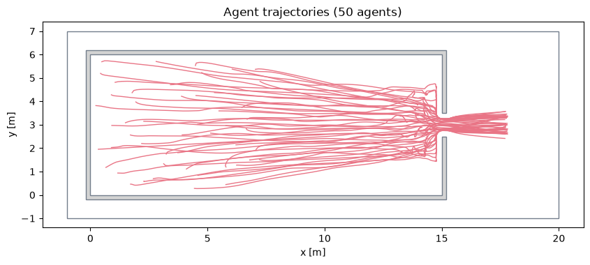
3. Plot the agent trajectories on the walkable area.

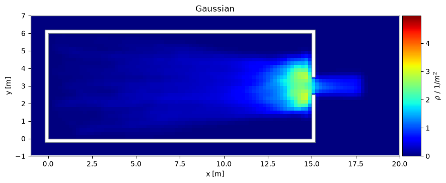
4. Compute a Gaussian density profile and render it as a time-averaged heatmap.

The scenario is the bottleneck export already shipped with the repo (examples/assets/bottleneck.zip).

1. Run the scenario and keep the SQLite

run_scenario(..., output_path=...) writes the trajectory to a path you control. We use a temp file so the notebook does not leave artifacts behind, but you can point this at any directory.

import logging
import tempfile
from pathlib import Path

logging.getLogger("jupedsim_scenarios").setLevel(logging.WARNING)

from jupedsim_scenarios import load_scenario, run_scenario

scenario = load_scenario("../assets/bottleneck.zip")

sqlite_path = Path(tempfile.mkdtemp()) / "bottleneck.sqlite"
result = run_scenario(scenario, seed=42, output_path=str(sqlite_path))

print(f"model           : {scenario.model_type}")
print(f"evacuation_time : {result.evacuation_time:.2f} s")
print(f"agents          : {result.agents_evacuated} / {result.total_agents}")
print(f"trajectory file : {sqlite_path}")

model           : CollisionFreeSpeedModel
evacuation_time : 53.18 s
agents          : 50 / 50
trajectory file : /tmp/tmp7vz3eg4p/bottleneck.sqlite

2. Read the trajectory with pedpy

pedpy ships native readers for the JuPedSim trajectory SQLite. They return a TrajectoryData (frames, agent ids, positions) and a WalkableArea (the simulation geometry), which all subsequent pedpy analysis functions consume directly.

from pedpy import (
    load_trajectory_from_jupedsim_sqlite,
    load_walkable_area_from_jupedsim_sqlite,
)

trajectory = load_trajectory_from_jupedsim_sqlite(trajectory_file=sqlite_path)
walkable_area = load_walkable_area_from_jupedsim_sqlite(trajectory_file=sqlite_path)

df = trajectory.data
print("columns       :", list(df.columns))
print("rows          :", len(df))
print("unique agents :", df['id'].nunique())
print("frame range   :", df['frame'].min(), "→", df['frame'].max())
print("walkable bbox :", walkable_area.polygon.bounds)

columns       : ['frame', 'id', 'x', 'y', 'point']
rows          : 15044
unique agents : 50
frame range   : 0 → 531
walkable bbox : (-1.0, -1.0, 20.0, 7.0)

3. Plot the trajectories

Each agent contributes one polyline. The walkable area is drawn as the underlying polygon so the trajectories sit in their geometric context.

import matplotlib.pyplot as plt
from pedpy import plot_trajectories

fig, ax = plt.subplots(figsize=(10, 4))
plot_trajectories(traj=trajectory, walkable_area=walkable_area, axes=ax)
ax.set_aspect("equal")
ax.set_xlabel("x [m]")
ax.set_ylabel("y [m]")
ax.set_title(f"Agent trajectories ({df['id'].nunique()} agents)")
plt.show()

4. Gaussian density profile

compute_density_profile returns one density grid per frame. With DensityMethod.GAUSSIAN each agent is smeared by a Gaussian kernel of the given full-width-at-half-maximum (gaussian_width), so the result is a smooth field rather than a step function.

We compute the profile across the entire run, then render it with pedpy’s plot_profiles, which averages the per-frame grids and overlays the walkable-area outline. The peak sits at the bottleneck entrance, as expected.

import numpy as np
from pedpy import DensityMethod, compute_density_profile

grid_size = 0.2  # metres per cell

gaussian_density_profile = compute_density_profile(
    data=df,
    walkable_area=walkable_area,
    grid_size=grid_size,
    density_method=DensityMethod.GAUSSIAN,
    gaussian_width=0.5,
)

profile_stack = np.asarray(gaussian_density_profile)
print("profile shape (frames, rows, cols):", profile_stack.shape)
print("peak density:", profile_stack.max(), "ped/m²")

profile shape (frames, rows, cols): (532, 40, 105)
peak density: 5.1350090155130355 ped/m²

from pedpy import plot_profiles

fig, ax = plt.subplots(figsize=(10, 4))

cm = plot_profiles(
    walkable_area=walkable_area,
    profiles=gaussian_density_profile,
    axes=ax,
    label=r"$\rho$ / 1/$m^2$",
    vmin=0,
    vmax=float(profile_stack.max()),
    title="Gaussian",
)
ax.set_xlabel("x [m]")
ax.set_ylabel("y [m]")
plt.show()

5. Clean up

We persisted the SQLite to a temp path ourselves, so we remove it explicitly. (When output_path is omitted, result.cleanup() would handle the temp file managed by the runner.)

sqlite_path.unlink(missing_ok=True)
sqlite_path.parent.rmdir()

Where to next

• pedpy has analogous helpers for flow, velocity, fundamental diagrams, and Voronoi density — they consume the same TrajectoryData / WalkableArea pair.

• For parameter studies, swap run_scenario for run_sweep and loop pedpy analysis over SweepResult.trials (see the 10_sweep_save_load how-to).

• For animated trajectories, pedpy’s plot_trajectories accepts TrajectoryData directly.