

Bottleneck N-T Diagram With Zone Speed Factor#
This notebook runs the shared community bottleneck example twice and compares the resulting \(N\)-\(T\) diagrams at the bottleneck throat.
Run 1 uses zone
speed_factor = 1.0Run 2 uses zone
speed_factor = 0.5
The final plot shows both runs side by side using pedpy.plot_nt(..., axes=...).
import logging
from datetime import datetime

# Silence jupedsim-scenarios' INFO/DEBUG output. See the howto
# "How do I inspect a scenario?" for the full list of levels.
logging.getLogger("jupedsim_scenarios").setLevel(logging.WARNING)

print(f"Executed on {datetime.now().strftime('%d.%m.%Y, %H:%M')}")

from pathlib import Path

import matplotlib.pyplot as plt
import pedpy

from jupedsim_scenarios import load_scenario, run_sweep
Executed on 05.09.2026, 10:15
SCENARIO_DIR = Path("scenario_files") / "bottleneck-zone"
MEASUREMENT_LINE = pedpy.MeasurementLine([(10.0, 4.5), (10.0, 5.5)])

scenario = load_scenario(str(SCENARIO_DIR))
scenario.summary()
'Scenario: /home/runner/work/jupedsim-scenarios/jupedsim-scenarios/docs/source/notebooks/cookbook/scenario_files/bottleneck-zone\n Model: CollisionFreeSpeedModel\n Seed: 42\n Max time: 300s\n Exits: 1\n Distributions: 1\n Stages: 0\n Zones: 1\n Journeys: 1\n Agents: ~50\n Journey elems: 2\n Route: 1 distribution, 0 checkpoint, 1 exit\n Sequence: jps-distributions_0 -> jps-exits_0\n jps-distributions_0: 50 agents'
Helper Functions#
We deep-copy the loaded scenario data before changing the zone speed factor. This keeps the baseline and modified runs independent, because nested edits to scenario.raw would otherwise leak into later runs.
def _nt_from_trial(trial):
    """Post-process one run_sweep trial into the rich dict the
    downstream cells expect (trajectory, n(t) curve, crossing frames).
    """
    traj = pedpy.TrajectoryData(
        trial.result.trajectory_dataframe()[["id", "frame", "x", "y"]],
        frame_rate=trial.result.frame_rate,
    )
    nt, crossing_frames = pedpy.compute_n_t(
        traj_data=traj,
        measurement_line=MEASUREMENT_LINE,
    )
    return {
        "speed_factor": trial.axis_values["speed_factor"],
        "result": trial.result,
        "trajectory": traj,
        "nt": nt,
        "crossing_frames": crossing_frames,
    }
Baseline Run#
First run the bottleneck with zone speed_factor = 1.0.
%%capture
# Sweep both speed_factor values through one run_sweep call so the two
# variants execute in parallel (workers=2) and share the per-trial
# .copy()/.cleanup() bookkeeping.
sweep = run_sweep(
    scenario,
    axes={"speed_factor": [1.0, 0.5]},
    apply={
        "speed_factor": lambda s, v: s.set_zone_speed_factor(0, float(v)),
    },
    seeds=[42],
    workers=2,
)
baseline = _nt_from_trial(sweep.trials[0])
slow_zone = _nt_from_trial(sweep.trials[1])
baseline["result"].metrics
INFO - Using fallback logic: No journeys defined
INFO - Processing with parameters: {'number': 50, 'radius': 0.15, 'v0': 1.2, 'distribution_mode': 'by_number', 'radius_distribution': 'constant', 'v0_distribution': 'constant'}
INFO - Using default parameters: v0=1.2, radius=0.15, n_agents=50
INFO - Distribution jps-distributions_0: {'number': 50, 'radius': 0.15, 'v0': 1.2, 'distribution_mode': 'by_number', 'percentage': None, 'use_flow_spawning': False, 'flow_start_time': 0, 'flow_end_time': 10, 'strict_spawning': False, 'use_premovement': False, 'premovement_distribution': 'gamma', 'premovement_param_a': None, 'premovement_param_b': None, 'premovement_seed': None, 'radius_distribution': 'constant', 'radius_std': None, 'v0_distribution': 'constant', 'v0_std': None}
INFO - Added 50 agents using fallback logic (immediate), prepared 0 flow sources
INFO - Using fallback logic: No journeys defined
INFO - Processing with parameters: {'number': 50, 'radius': 0.15, 'v0': 1.2, 'distribution_mode': 'by_number', 'radius_distribution': 'constant', 'v0_distribution': 'constant'}
INFO - Using default parameters: v0=1.2, radius=0.15, n_agents=50
INFO - Distribution jps-distributions_0: {'number': 50, 'radius': 0.15, 'v0': 1.2, 'distribution_mode': 'by_number', 'percentage': None, 'use_flow_spawning': False, 'flow_start_time': 0, 'flow_end_time': 10, 'strict_spawning': False, 'use_premovement': False, 'premovement_distribution': 'gamma', 'premovement_param_a': None, 'premovement_param_b': None, 'premovement_seed': None, 'radius_distribution': 'constant', 'radius_std': None, 'v0_distribution': 'constant', 'v0_std': None}
INFO - Added 50 agents using fallback logic (immediate), prepared 0 flow sources
Slowdown Run#
Now change the zone speed factor to 0.5 and rerun.
slow_zone["result"].metrics
{'success': True,
 'status': 'completed',
 'message': 'All agents evacuated before reaching the maximum simulation time.',
 'evacuation_time': 56.22,
 'total_agents': 50,
 'agents_evacuated': 50,
 'agents_remaining': 0,
 'all_evacuated': True,
 'frame_rate': 10.0,
 'dt': 0.01,
 'seed': 42,
 'walkable_polygon': <POLYGON ((0 0, 10 0, 10 4.5, 15 4.5, 15 0, 25 0, 25 10, 15 10, 15 5.5, 10 5...>}
Geometry, Zone, and Trajectories#
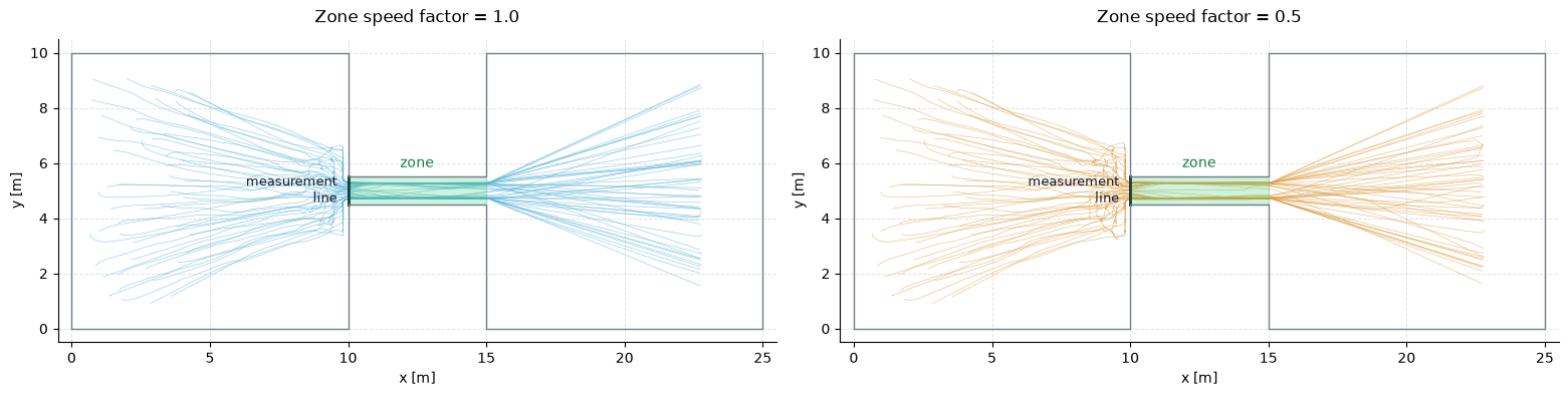
The panels below show the bottleneck geometry, the slowdown zone polygon, the measurement line, and the trajectories for both runs.
zone_xy = scenario.raw["zones"]["jps-zones_0"]["coordinates"]

fig, axes = plt.subplots(1, 2, figsize=(15.5, 5.8), constrained_layout=True)

for ax, run, color in [
    (axes[0], baseline, pedpy.PEDPY_BLUE),
    (axes[1], slow_zone, pedpy.PEDPY_ORANGE),
]:
    pedpy.plot_measurement_setup(
        traj=run["trajectory"],
        walkable_area=pedpy.WalkableArea(scenario.walkable_polygon),
        measurement_lines=[MEASUREMENT_LINE],
        axes=ax,
        traj_alpha=0.72,
        traj_width=0.4,
        ml_width=2,
        ml_alpha=0.28,
        traj_color=color,
        ml_color="#111827",
    ).set_aspect("equal")
    ax.fill(
        [xy[0] for xy in zone_xy],
        [xy[1] for xy in zone_xy],
        color="#22C55E",
        alpha=0.22,
        zorder=2,
    )
    ax.text(12.5, 5.85, "zone", color="#15803D", fontsize=10, ha="center")
    ax.text(9.6, 5.0, "measurement\nline", color="#111827", fontsize=9, ha="right", va="center")
    ax.set_title(f"Zone speed factor = {run['speed_factor']:.1f}", pad=12)
    ax.set_xlim(-0.5, 25.5)
    ax.set_ylim(-0.5, 10.5)
    ax.set_xlabel("x [m]")
    ax.set_ylabel("y [m]")
    ax.grid(True, linestyle="--", linewidth=0.7, alpha=0.35)
    ax.spines["top"].set_visible(False)
    ax.spines["right"].set_visible(False)

plt.show()
Side-By-Side N-T Diagrams#
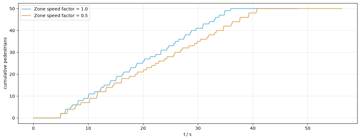
The slower zone should delay cumulative crossings at the measurement line.
fig, axes = plt.subplots(1, 1, figsize=(14, 5))

pedpy.plot_nt(
    nt=baseline["nt"],
    axes=axes,
    label="Zone speed factor = 1.0",
    color=pedpy.PEDPY_BLUE,
)

pedpy.plot_nt(
    nt=slow_zone["nt"],
    axes=axes,
    label="Zone speed factor = 0.5",
    color=pedpy.PEDPY_ORANGE,
)
axes.legend()
axes.grid(alpha=0.3)
Cleanup#
Delete the temporary SQLite files when you are done.
baseline["result"].cleanup()
slow_zone["result"].cleanup()
1